GARCHの初歩への道
GARCH(1,1)とGARCH-Mの初歩
This presents garch(1,1) and garch-M using


	simple R code examples
GARCH(1,1)とGARCH-M の入門的なモデルの推定についてまとめてみた。
登山にたとえれば、山岳ガイドが登山口で基本的事項を説明するようなものではなく、最寄り駅に降り立った登山客に行きずりの人が登山口はあちらの方ですよと話すような内容となっている。
Forecasting: principles and practiceという専門書が https://otexts.com/fpp2/ で公開されているが、ボラティリティモデルは扱われていない。
ここでは最も単純なGARCH(1,1)モデルの適用についてrugarchを使って検討してみる。GARCH過程はARCH過程を一般化したもので、GARCH(1,1)は条件付分散をhで表しhは1期前の誤差の2乗と1期前のh(ボラティリティをも意味する)に依存する形となっている。
GRACH(1,1)について
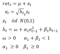
収益率retの誤差項eが以下の条件に従って時間と共に変動するモデルGARCH(1,1)を考える。数式でまとめると以下のようになる。
株式収益率のデータについてGARC(1,1)のモデルをあてはめてみる。
length(SP500)
## [1] 2780
ret<-ts(SP500)
garchspec1 <- ugarchspec(
##
## *---------------------------------*
rhat1 <- garchFit1@fit$fitted.values
plot.ts(rhat1,ylim = c(-1, 1))
	推定結果は以下のようになり,係数の推定値はt値が大きく有意となっている。μ= 0.0553 ω= 0.0043
	α=0.0478 β= 0.9481
ret=0.0553 + 誤差
h(t)=0.0043+ 0.0478×誤差(t-1)^2 + 0.9491×h(t-1)
と推定されている。無条件分散は ω/(1-α-β)≒ 1.048
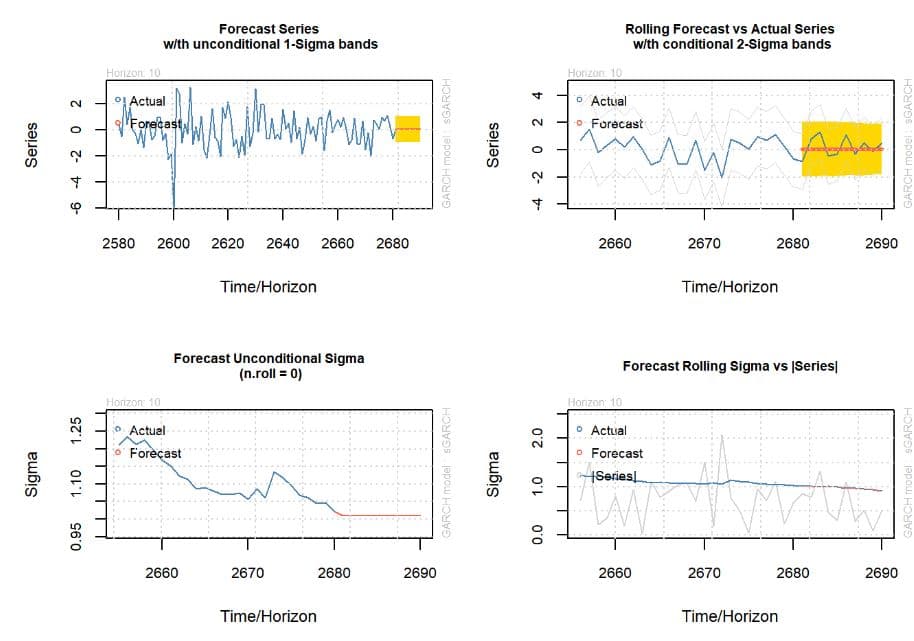
rugarchには予測モデルも作れるので,10期先までの単純な予測を試みると以下のようになる。
	 fmodel
	<- ugarchforecast(garchFit1,n.roll=10,n.ahead=10,data=ret)
	plot(fmodel,which="all")
GARCH-M(GARCH in MEAN)モデル
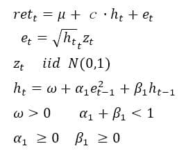
収益率retの誤差項eが以下の条件に従って時間と共に変動するモデルGARCH-M(GARCH in MEAN)を考える。retの平均式の中に説明変数として条件付分散が#付け加わったモデルである。
現代ポートフォリオ理論に従ってリスクが高まればより大きな収益率が求められるという関係を示している。
cは追加リスクに対応するリスクプレミアムを意味している。
数式でまとめると以下のようになる。
GARCH-Mモデルの平均式 retにはhが入っているが、hは系列相関をもっているので、hの影響を受けてretも系列相関をもち、結果的に収益率は過去の収益率の影響を受ける関係を表現している。
ugarchspecの中のarchmは説明変数として条件付分散が入ることを示し、archpowは分散か標準偏差の何れかの形で説明変数にするかを表す。説明変数にhを使うときにはarchpow=2は分散、h^0.5 つまり標準偏差を使うときにはarchpow=1 と指定する。
garchSpec2 <-
ugarchspec(mean.model=list(armaOrder=c(0,0), archm=T,archpow=2),
distribution.model="norm", variance.model=list(garchOrder=c(1,1))) garchm1 <
- ugarchfit(garchSpec2, data=ret) show(garchm1)
##
## *---------------------------------*
## * GARCH Model Fit *
## *---------------------------------*
##
## Conditional Variance Dynamics
## -----------------------------------
## GARCH Model : sGARCH(1,1)
## Mean Model : ARFIMA(0,0,0)
## Distribution : norm
##
## Optimal Parameters
## ------------------------------------
## Estimate Std. Error t value Pr(>|t|)
## mu 0.023875 0.023406 1.0201 0.307700
## archm 0.052718 0.032836 1.6055 0.108378
## omega 0.004879 0.001810 2.6948 0.007043
## alpha1 0.053868 0.008483 6.3505 0.000000
## beta1 0.942488 0.009144 103.0663 0.000000
##
## Robust Standard Errors:
## Estimate Std. Error t value Pr(>|t|)
## mu 0.023875 0.024121 0.98979 0.322274
## archm 0.052718 0.035390 1.48966 0.136314
## omega 0.004879 0.002893 1.68645 0.091709
## alpha1 0.053868 0.015657 3.44063 0.000580
## beta1 0.942488 0.016832 55.99247 0.000000
##
## LogLikelihood : -3478.7
##
## Information Criteria
## ------------------------------------
##
## Akaike 2.5062
## Bayes 2.5169
## Shibata 2.5062
## Hannan-Quinn 2.5101
##
## Weighted Ljung-Box Test on Standardized Residuals
## ------------------------------------
## statistic p-value
## Lag[1] 6.738 0.009438
## Lag[2*(p+q)+(p+q)-1][2] 6.746 0.013926
## Lag[4*(p+q)+(p+q)-1][5] 12.752 0.001766
## d.o.f=0
## H0 : No serial correlation
##
## Weighted Ljung-Box Test on Standardized Squared Residuals
## ------------------------------------
## statistic p-value
## Lag[1] 0.2063 0.6497
## Lag[2*(p+q)+(p+q)-1][5] 3.1770 0.3757
## Lag[4*(p+q)+(p+q)-1][9] 3.8997 0.6059
## d.o.f=2
##
## Weighted ARCH LM Tests
## ------------------------------------
## Statistic Shape Scale P-Value
## ARCH Lag[3] 0.2614 0.500 2.000 0.6092
## ARCH Lag[5] 0.3388 1.440 1.667 0.9298
## ARCH Lag[7] 0.7099 2.315 1.543 0.9556
##
## Nyblom stability test
## ------------------------------------
## Joint Statistic: 0.9512
## Individual Statistics:
## mu 0.1997
## archm 0.1501
## omega 0.1697
## alpha1 0.3798
## beta1 0.2375
##
## Asymptotic Critical Values (10% 5% 1%)
## Joint Statistic: 1.28 1.47 1.88
## Individual Statistic: 0.35 0.47 0.75
##
## Sign Bias Test
## ------------------------------------
## t-value prob sig
## Sign Bias 0.9817 0.32632
## Negative Sign Bias 1.3957 0.16292
## Positive Sign Bias 1.8310 0.06721 *
## Joint Effect 19.3632 0.00023 ***
##
##
## Adjusted Pearson Goodness-of-Fit Test:
## ------------------------------------
## group statistic p-value(g-1)
## 1 20 72.09 4.125e-08
## 2 30 84.12 2.849e-07
## 3 40 100.09 2.849e-07
## 4 50 112.27 7.160e-07
##
##
## Elapsed time : 0.41705
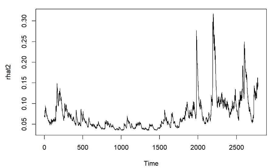
rhat2 <- garchm1@fit$fitted.values
plot.ts(rhat2)
hhat2 <- ts(garchm1@fit$sigma^2)
plot.ts(hhat2)
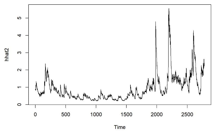
推定結果は以下のようになり、μ= 0.0238 c=0.0527
ω= 0.0048 α=0.0538
β= 0.9424
ret=0.0238 + 0.0527×h + 誤差 h(t)=0.0048+ 0.05388×誤差(t-1)^2 + 0.9424×h(t-1)
と推定されている。
GARCH-Mモデルでは収益率も大きく変動していることが
グラフで分かる。GARCH(1,1)モデルでは平均値で一定だったが収益率がhの影響を受けるのでGARCH-Mではボラタイルとなってる。
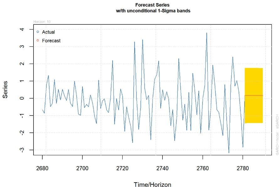
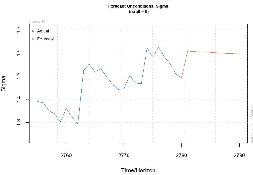
rugarchには予測モデルも作れるので,10期先までの単純な予測を#試みると以下のようになる。
fmodel <- ugarchforecast(garchm1,n.roll=0,n.ahead=10,data=ret)
plot(fmodel,which=c(1))
plot(fmodel,which=c(3))
rolling予測も出来るが、その場合は予測に100個のデータを使うのでout.sample=100 を指定しておく。rolling forecastについては
garchFit3 <- ugarchfit(spec=garchSpec2, data=ret,out.sample=100)
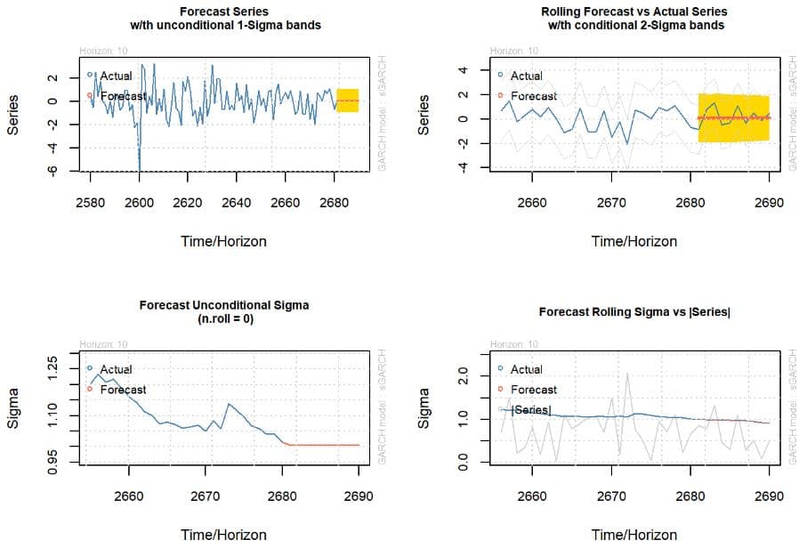
rugarchにはブートストラップ法で予測する機能もついているので10期先までの予測を試みると以#method=c("Partial")でなくc("Full")も指定できるが、RのバージョンがR-4.0.2 だとエラーとなってしまう。R-3.6.2の時にはc("Full")を指定しても少々時間がかかるが計算してくれる。ちなみにrugarchのバージョンは1.4.0
を使用している。
bootp<- ugarchboot(garchm1,method=c("Partial"),n.ahead =
                                                        10,n.bootpred=100,n.bootfit=100)


bootp
##
## *-----------------------------------*
## * GARCH Bootstrap Forecast
*
## *-----------------------------------*
## Model : sGARCH
## n.ahead : 10
## Bootstrap method: partial
## Date (T[0]): 2780-01-01
##
## Series (summary):
## min
q.25 mean q.75
max forecast[analytic]
## t+1 -4.5047 -1.15111 0.001599 0.75044 5.0786
0.16023
## t+2 -2.9764 -0.65115 0.191981 1.17784 3.6243
0.15999
## t+3 -6.9669 -0.66939 0.212311 1.27388 4.9540
0.15976
## t+4 -3.1171 -0.46887 0.474701 1.33241 4.3096
0.15952
## t+5 -3.9732 -0.63170 0.119738 1.12066 3.7115
0.15928
## t+6 -3.9451 -0.48926 0.169970 1.19663 3.6684
0.15905
## t+7 -7.5622 -1.11045 -0.225839 0.68351 6.3595
0.15881
## t+8 -6.4267 -1.05151 -0.116018 0.81089 4.2977
0.15858
## t+9 -9.0114 -0.85119 0.023165 1.02170 4.9233
0.15834
## t+10 -4.0601 -0.63714 0.113709 0.96303 5.0671
0.15811
## .....................
##
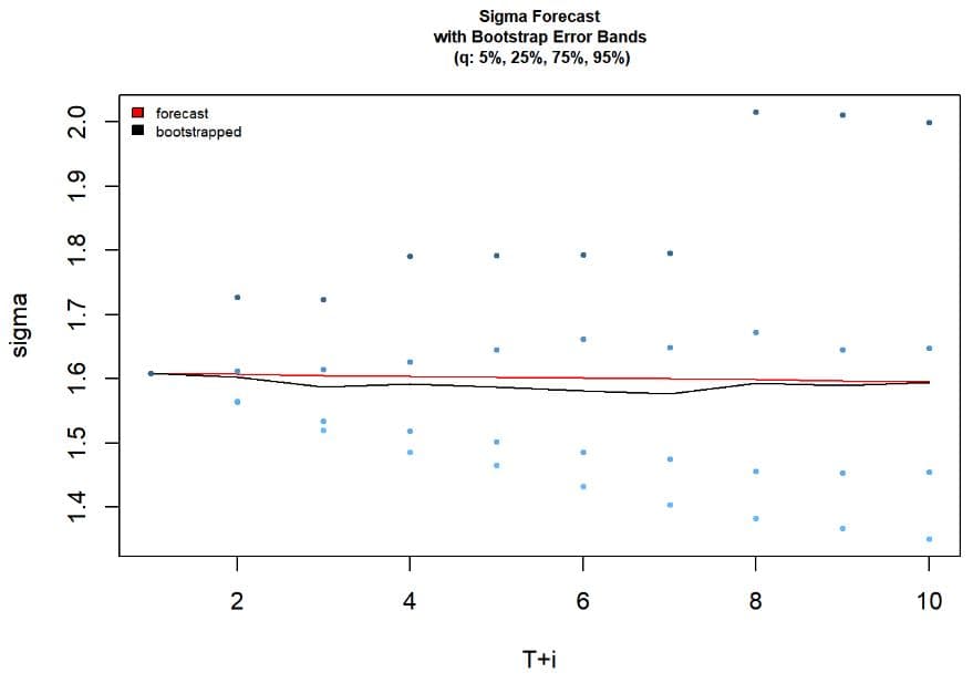
## Sigma (summary):
## min q0.25
mean q0.75 max forecast[analytic]
## t+1 1.6083 1.6083 1.6083 1.6083 1.6083
1.6083
## t+2 1.5629 1.5643 1.6031 1.6127 1.9354
1.6069
## t+3 1.5192 1.5340 1.5878 1.6141 1.9043
1.6055
## t+4 1.4775 1.5184 1.5924 1.6260 2.2347
1.6041
## t+5 1.4441 1.5021 1.5868 1.6447 2.1820
1.6027
## t+6 1.4108 1.4857 1.5817 1.6618 2.1195
1.6013
## t+7 1.3939 1.4752 1.5762 1.6486 2.0811
1.5999
## t+8 1.3558 1.4553 1.5930 1.6727 2.4105
1.5985
## t+9 1.3243 1.4532 1.5894 1.6449 2.4745
1.5971
## t+10 1.2892 1.4551 1.5939 1.6481 2.6021
1.5957
## .....................plot(bootp,which=c(2))
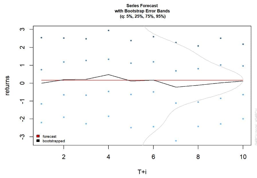
plot(bootp,which=c(3))
最尤法とRのコーディングについて
最尤法の基本的な仕組みについては 最尤法の考え方を簡単な計算例で探求 with R で簡単にまとめてみた。
AIが普及し始めてからコーディングの仕方も大きく変わり、RStudioもCopilotと連係して便利であった。
Copilotが有効化されているとプログラムを書き始めると影法師のように薄い色の文字(ghost
text)が表示されコードの作成を先読みしてコードの提案をしてくれた。Copilotの提案が気に入ればTabキーを押すと確定した文字に変わり、そのままコードとして使えるのでプログラムが作成しやすかった。
しかし、このAI機能は便利だと思っていたが、2026年4月頃から様子が変わりRStudio2026.04ではAI機能は有料化されたようだ。AI機能は
Posit AIとGitHub Copilotが選択できるが月額料金を支払う必要があるようだ。現在のところ、契約をしていないのでAI機能は
使えない状態となっている。世の流れとして今まで無料で使えた物が従量課金に変わっていくように感じる。
AIの回答が御門違いとか物足りなさを感じることが多くなったときには、最初に一か月だけ有料バージョンを使ってみて
満足がいくものであれば有料バージョンに切り換えようかと思案している。例えば、ピタゴラスの定理の証明を質問すると無料版ではネットで解説されている
一般的な証明を解説するので、それで十分であれば無料バージョンで支障は無いだろう。ただ、上位バージョンだと幾何、代数、解析学などで多種類の証明を提示できるそうだ。もし、そのような回答が必要になれば切換の時期かもしれないと思っている。最近、標準正規分布関数(累積分布)と誤差関数(Erf function)の変換公式の証明を置換積分を使って、無料のAIが丁寧に解説してくれたので、自分にとって何時、有料バージョンに切り換えるのか全く想像もできないでいる。
GitHub Copilotの有料化については
https://github.blog/jp/2026-04-28-github-copilot-is-moving-to-usage-based-billing/
を参照